GitHub - Kongstad/Geo_Project_TensorFlow: Repository for semester course on using TensorFlow for image recognition of satellite imagery.

Project name:

Geological Project - Investigating the use of Google TensorFlow for image recognition of satellite imagery.

Student info:

Name: Peter Kongstad
Field of study: Geoscience - 8th semester
University: Aarhus University
Contact: [email protected]
Primary Supervisor: Christoffer Karoff - Department of Geoscience & Department of Physics.
Secondary Supervisor: Rune Hylsberg - Department of Engineering.

Project description:

This is a repository for my semester project on using Google TensorFlow for Deep Neural Network learning, Raster Vision for object detection on GeoJSON files, Rasterio for data handling and several modules. The end goal is to test the software and conclude on wether or not it is the desireable choice for the follow-up project, of which is my master thesis. Through this document, I've written the "how-to's" and given conclusions on the individual software, as well as documenting the complications that arose. A conlusion on this feasibility study can be found at the bottom of this page.

Software introduction:

Anaconda Navigator

Information
Anaconda makes it easier to create and manage python environments as desired. Therefore it can be useful for setting up a primary environment, with the most basic required modules installed for TensorFlow applications. Then this environment can be cloned for experimental purposes without the risk of jeopardizing the primary environment. Besides managing the python environment, this software is also very useful in terms of adding new modules and installing the Spyder IDE and Jupyter Notebook. It is not an essential product, but definitely a useful one.
CUDA

Information
CUDA (Compute Unified Device Architecture) is a parallel computing platform and programming model developed by Nvidia which provides an API to the parallel computing capabilities of GPU. It has been proven that the training of DNNs can be significantly accelerated using parallel computing. This is essential to be able to try out different architectures and compare their performance. In this project, an Nvidia 1080 GPU is used. More information can be found at Nvidia's CUDA Zone
cuDNN

Information
cuDNN is a shortened form of CUDA Deep Neural Network library. It is a library for deep neural networks which provides GPU accelerated functionality. This library provides implementations for the common methods of DNN, such as convolutional, normalization and pooling layers, different activation functions and the most common optimization algorithms. This library streamlines processes of optimization, as the utilization of the GPU is already set up and configured to run with Tensorflow. This is essential to the project, as we otherwise would have to manually setup low-level processes in the GPU, which would require high-level knowledge about data and processor functionality. Besides, Tensorflow is already configured to perform efficiently with this library. According to Nvidia's developer page, the newest version of 7.0 and above, which is used in this project, have 3x faster training performance than previous versions.
Python 3.6

Information
Python is an interpreted, object oriented, high-level programming language. It has a wide array of usages and is very often utilized in our field by scientist and researchers, but can readily be applicable by anyone. Python is relatively simple and fast programming language with a manageable learning curve. For this project version 3.6 is used. This version is the most recent major release and has proven it self to be stable and greatly backed by a large number of modules. TensorFlow recommends using Python3.5 and above for GPU-supported application.
TensorFlow

Information
TensorFlow is an open-source software library for computation and displaying data flow graphs. The software architecture is very flexible, meaning that it allows for computation between several platforms such as CPU's, GPU's and TPU's(Tensor Processing Unit). Besides spanning platforms, it also allows for distributing the mathematic load over several desktops to clusters of servers and even mobile devices. TensorFlow is generally build for machine learning and deep learning, and the software is already widely applied across scientific branches. Since TensorFlow is able to display graphs of the structure of the models being build, it is easier to get the full overview of a given model. The graph is a data structure which describes the computation that a model performs. Thus it is easier to discern an outcome, study it and fine tune further development of the model. TensorFlow already provides several pre-trained models on their GitHub page. These models can be freely downloaded and applied. I have demonstrated the use of one of these pre-trained modules, in the iceberg object detection example, which is discussed further down this page.
Spyder IDE

Information
Spyder is an open source cross-platform Integrated Development Environment, tailored for scientific programming in conjunction with the Python language. It comes with advanced editing, interactive testing and debuggig. Spyder also hosts a numerical computing environment, due to the support of IPython, which is an enhanced interactive python interpreter. Spyder further integrates well-known modules such as NumPy(Linear Algebra), SciPy(Signal and image processing), Matplotlib(interactive 2D/3D plotting) and much more. It is also an integral part of the Anaconda Navigator, which allows for easy interplay between environments and Spyder can therefore be installed into each environment as required.

Project Timeline:

February 2018:

Project startup approved
Basic TensorFlow tutorials completed
Initial progress documented in /files/process.pdf

March 2018:

Complete hardware reset and reinstallation to bypass previous issues - See process.docx.
TensorFlow succesfully operational with GPU Support:
- OS: Linux Ubuntu 16.04
  
  Modification
  
  A slight modification in the Software & Updates panel is required. In the sub-menu Additional drivers, I had to disable the Ubuntu Nouveau display driver and instead set it to: Using Nvidia binary - driver. This makes sure that there is no driver conflict.
- Anaconda Navigator: 4.5.0
  
  Installation
  
  Anaconda Navigator was downloaded from their website and thereafter updated to version 4.5.0 by using the navigator automatic updating platform.
- CUDA: 9.0
  
  Installation
  
  I've proceeded to the CUDA 9.0 website to download this specific version, as it should work better with this setup. I've downloaded CUDA 9.0 from here. I've chosen the Linux version, with x86_64, for Ubuntu 16.04 and the installer as a deb(local) type. Then I've launched the following terminal commands for download and correct installation
  1. Set the directory to the folder with the downloaded CUDA file.
  2. sudo dpkg -i cuda-repo-ubuntu1604-9-0-local_9.0.176-1_amd64.deb
  3. sudo apt-key add /var/cuda-repo-9-0-local/7fa2af80.pub
  4. sudo apt-get update
  5. sudo apt-get install cuda
  I then proceed to the CUDA installation documentation, which states at point 7.1, that some actions must be taken after the installation before the CUDA Toolkit and Driver can be used.
  The PATH variable needs to include /usr/local/cuda-9.1/bin, so to add this path to the PATH variable, the following command needs to be entered in the terminal window:
  export PATH=/usr/local/cuda-9.1/bin${PATH:+:${PATH}} In addition, when using the runfile installation method, the LD_LIBRARY_PATH variable needs to contain /usr/local/cuda-9.1/lib64 on a 64-bit system.To change the environment variables for 64-bit operating systems, enter the following in a terminal window:
  export LD_LIBRARY_PATH=/usr/local/cuda-9.1/lib64
  ${LD_LIBRARY_PATH:+:${LD_LIBRARY_PATH}} The installation can then be verified by typing the following into a terminal window: "nvcc -V".
- cuDNN: 7.0.5
  
  Installation
  
  In order to download cuDNN, a Nvidia developer membership is required. This can freely be obtained by simply registrating on their website. I've done so and proceed to download the file at this website. The file I've used for this is the one labelled cuDNN v7.0.5 Runtime Library for Ubuntu16.04 (Deb). Once this file is downloaded. I double click it to initiate the software installer.
- Python: 3.6
  
  Installation
  
  I have installed python3.6 through Anaconda Navigator by creating a new python environment in the Anaconda directory, to install TensorFlow into - which I named tensorflow. This was done by the using the command "conda create -n tensorflow pip python=3.6" . I then activate the newly created environment by typing source activate tensorflow. I then launch the Anaconda Navigator and install the Spyder editor in the tensorflow environment. With Anaconda now all set up, Tensorflow can be installed
- TensorFlow:
  
  Installation
  
  Now in order to install Tensorflow, I use the following terminal command to install the GPU supported version pip install --ignore-installed --upgrade https: //storage.googleapis.c om/tensorflow/linux/gpu/tensorflow_gpu-1.6.0-cp36-cp36m-linux_x86_64.whl Note that this is the correct TensorFlow for python 3.6, by its denomination cp36.
- Spyder Test:
  
  Code Compilation
  
  In order to test whether TensorFlow is sucessfully working, I now compile a short "Hello, TensorFlow" test as given here.
  The code looks like this:
  #Python
  import tensorflow as tf
  hello = tf.constant('Hello, TensorFlow!')
  sess = tf.Session()
  print(sess.run(hello))
  Which succesfully prints
  'Hello, TensorFlow!'

April 2018:

May 2018:

Satellite Imagery Challenges

Information
The initial technique of using the Sentinelsat API tool for image retrieval, seems to be undesirable at this point in time. There are three major hurdles in using this technique so far. 1) The immense file size of requesting 1 photo at a given location. In these zipped folders, there are all 13 bands, as well as several datafiles. This can easily produce file sizes above 1.3 gb. When in reality the desired product was an image at the size of 122 mb. 2) ESA throttles their servers download speed. Putting a 1.3 gb file download time to more than 30 minutes, at a very reasonable broadband connection (50/50 mbit). They are simply limiting the outgoing server speeds. 3) The images are often extremely bright as a product of the snow albedo. Image brightness can ofcourse be reduced. Conclusion: I suggest for this pilot project, that the focus is on getting the image recognition going, rather than dealing with image retrieval and editing technicalities. Hence I've concluded it is better to use their online sentinel hub website (EO Browser). The images I require can be loaded up in less than 10 seconds and several parameters can be defined. Such as format, with or without georeference, quality, coordinate system and band/layers. I've decided to proceed with this method. 15 images have been selected so far and can be found here /Files/images/.
Image recognition methods used on ice sheet images
- TensorFlow Image Recognition by ImageNet
  
  Information
  I've used the image classifier tutorial listed on the TensorFlow website and then applied their code to the retrieved satellite imagery. This is a simple test where only 1 image is chosen, then compared to a large online database. The trick here is for TensorFlow to categorise as much as possible, then listing the top 5 objects and how often the algorithm guessed it right - Actually the error % rate. Testing on several images, it was able to say that the image contained icebergs and seashores. However it also misclassified other objects as killer whales, geysers and a Newfoundland Dog. To the algorithms credit, it guessed the seashore wrong only 2 % of the time. I've uploaded a Jupyter Notebook about with a little more details. It can be found at /Files/jupyter-notebooks/TF_IR_tut.ipynb
- Object Detection in action
  
  Information
  I have changed the object detection tutorial as provided by the RasterVision library to run a satellite image with a large ice sheet flowing. Initially it was problematic as the models didn't seem to recognize anything, as it did in the demo tutorial (the object detection tutorial notebook mentioned earlier). I realised a different model was required and tried changing between several different models. These models can be found at the TensorFlow github page right here. By switching the model to "faster_rcnn_inception_resnet_v2_atrous_oid_2018_01_28", I was finally able to get the large icesheet framed. I've produced a jupyter notebook of it which can be found at /Files/jupyter-notebooks/TF_IR_tut.ipynb
Follow-up investigation
- Semantic Segmentation vs. Object recognition
  
  Information
  For this project I've investigated both semantic segmentation and object recognition. For simplicity the object recognition seems at first to be the easiest method. By simply creating a bounding box around the ice in the images. However, for the follow-up project, it seems evident that the semantic segmentation is the way forward. This is due to the complexity of the follow up project. Whilst identifying 1 or 5 classes in a picture may be preferential in simplistic images. Working with large satellite imagery and trying to define small features, then pixelwise recognition may prove more fruitful. In comparision, visually, this means that when we want to detect an object, it will not be covered by a bounding box, but rather the entire object will be marked - pixel by pixel.
  Semantic segmentation works by understanding an image at the pixel level. Thus by assigning each pixel in an image to an object class.
- GPU vs. CPU
  
  Information
  Graphics Processing Units and Central Processing Units works in different ways, and therefore it is also situationally dependent, which one will perform best. Generally it can be said that CPUs handle algorithms such as GLMs better than a GPU would, and is generally more flexible. This is due to CPU's working more sequential. Where as the GPUs are parallelised and less flexible. This makes GPU preferential in machine learning cases such as with DNN. To go more in depth in understanding the difference, it is helpful to know the broadly simplified architecture of both processing units. A typical CPU is constructed for a more generic computing workload, as such that software is to be executed sequentially, implying one line/command at a time. However, this method places a limit to how fast a CPU can function. Secondly a CPU have fewer, but more complex cores to work with. Therefore CPU's do not function very well in gaming, multimedia application or with big data. This is where GPUs perform better with their parallelised architecture and large amount of simpler cores. The GPU are build as such, that it executes as many instructions as possible in parallel, but at the cost of slow sequential execution. GPU's primary weakness is memory capacity. Whilst they can draw a much higher memory bandwidth than a CPU, they tend to stretch the latency - meaning it is slower in transferring data. Another architectural difference is that CPU's are often clocked much higher than GPU's. Sequential tasks on a GPU is therefore not expected to match that of a CPU. The GPU provided for this project has 2560 CUDA cores, and can therefore computate massive amount of data, of the sort that can be parallelized (Matrix-matrix multiplications for example). This is why GPUs are significantly faster in deep learning applications. As mentioned this is just a broad overview of some cons and pros of the two types of processing units. A detailed description of this topic would exceed the scope of this report. The conlusion is that the GPU is simply able to juggle massive amounts of data simultaneously, in comparison to a CPU and therefore can shorten DNN methods down by days if not weeks, depending on the task. GPUs simply have more resources in form of its number of cores, its faster bandwidth to memory and the fact that DNN computations fit well with the GPU architecture.
- U-net Architecture
  
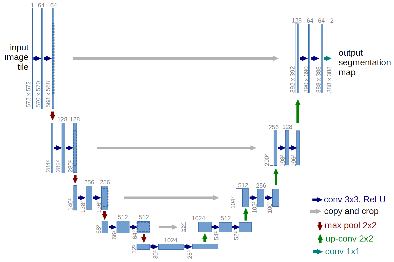
  Information
  U-Net architecture is a convolutional network architecture for quick and exact segmentation of images. It works by inputting a raw image and it essentially outputs a segmentation map of the image, highlighting features. One of the remarkable things about this architecture is, that the researchers who developed it for the biomedical field, was able to produce very good results with as few as 30 annotated images per application. The images also featured objects of the same class touching each other, in some cases overlapping or even with invisible borders, meaning that it was required that the model could distinguish and seperate these objects. The architecture of the convolutional network contains several convolutional and max pooling operations and can be seen here. The network is fed an image, then the data is propagated and resized along all possible paths through the multichannel feature maps, eventually producing a segmented output image with 2 classes. A background and foreground image. The structure is relatively complex and for the sake of understanding its setup, I've provided a link to a 5 minute video explaining the model in its entirety here. I strongly recommend watching it.
- QGIS
  
  Information
  QGIS is an cross-platform, open-sourced and free Geographic Information System(GIS) application. The software allows for the analysis and editing of geospatial data, and provides the tools for composing and exporting graphical maps. QGIS supports both raster and vector layers, allowing for drawing points and polygonal features on satellite imagery. It also supports a wide variety of raster image formats, can work with layers and it can manage georeferenced images. The software can, as with conventional GIS programs, combine geophysical data with map and satellite data. With the addition of local geophysical data retrieved from Greenland, added on top of Sentinel satellite images and possibly additional Digital Elevation Maps(DEM), it could be a powerful tool for combining all the data into a single comprehensible visual product. QGIS is also able to connect directly to python through plugins. Whether or not QGIS is entirely relevant for machine learning processes can be debated, but it could have potential in working with geologicals areas of interest and with pre-existing geological data.

Conclusion:

Introduction
For this feasibility project, I have utilized the TensorFlow DNN software and it’s associated products, enabling the usage of GPU support for faster calculation of the algorithms. This with the aim, of using Convolutional Neural Network techniques in image recognition. To start out with, I was tasked with making the TensorFlow software run along with its associated software and modules. Secondly I was tasked with testing out different methods of data retrieval and management, which I will conclude on in this section. Lastly I was to attempt simple image recognition of the satellite imagery obtained. Through this section I comment superficially on the important aspects and take-aways. For a more thorough comment on process, complications and solutions, check the individual points in the above section of this readme file.

Installation:
The first task of this project, was to get the GPU support up and running with TensorFlow, which is from here on denoted simply as “TF”. As there is little to no direct guidance provided by the TF team, this is not a trivial task. The different softwares have to be installed in a specific order, or conflict can arise. First step here was to make a system modification to the Linux Ubuntu setup, in order to avoid display driver conflict. Next was the installation of the CUDA 9.0 software, which enables the use of the Nvidia GPU in the TF module and associated modules. Also not a trivial task, but in this case, there was adequate documentation provided by Nvidia. The third requirement for the setup, was the cuDNN software. In order to utilize this software, which is an essential component, membership at the Nvidia developer page was required. Once obtained, the correct version could be installed without any hassle. Next requirement was the installation of Python 3.6 and creating the environment for the TF modules. Once the environment was configured, it was simple to install TF into this environment.

Data Import:
As my progress indicates in the sections above, there are several ways to retrieve the data. The simplest is by accessing the EO browser. This website offers an easy-to-use browser interface, where the desired parameters can easily be entered and then an output is generated in a equally easy to use format. The page requires registration and subsequently payment. However, new profiles with trial periods can be used. The second way is the proper way to do this, and in the follow-up project the way I would advice us to proceed. By utilizing the ESA Sentinel API, a script will connect directly to the ESA server and retrieve the images in bulk, provided the script feeds them a GeoJSON file with coordinates of the desired region. The image retrieval can be customized to a given preference dictated by parameters in the script. There are slight issues with this method though. The files are rather large, as all 13 bands and pre-processed images are contained within the file. Secondly the server is being throttled by ESA. Decreasing download speed severely. It would be interesting to consider approaching ESA and put in a request for a university pipe, that could offer increased download speeds. Regardless of this, I recommend we proceed with this method of obtaining Sentinel data. Especially for the L2A images.

Rasterio:
The Rasterio module is, as previously mentioned, a tool for importing and editing large Geo-imbedded satellite images. This module lived up to its expectations and was relatively easy to use. I’m not convinced this module is essential to the follow up project. However it does seem to make some image manipulation easier and thus faster, rather than have to do it manually. I would not sign this particular module off yet, neither would I declare it essential. I recommend keeping it in the toolbox for now.

RasterVision:
This module is under strong development and have changed entirely twice over this semester. This has made it slightly difficult to work with, since their github contents have changed over night. As it looks now, they are aiming at a major bundle release in the summer of 2018. Further investigation of their product reveals that they are working on releasing a stand-alone client, which seems to be their main focus. Regardless thereof, I was able to apply their previous image recognition code into one of the satellite images that I retrieved. By adjusting their initial model to a different TF released model, the code successfully identified a large ice sheet in a image and framed it. This proves what they are working on, works to a certain degree. However, after consulting PhD. Jacob at Engineering, I was advised to look in a different direction. Rather than using Object Orientated recognition, which RasterVision now specializes in, I was advised to investigate the Semantic Segmation method. Upon following this direction, I must concur with Jacob. By semantically segmented images, the image is divided up into pixels which are then assigned classes. This allows for creating pixel wise boundaries in the satellite images. Giving incredible precision. I’ve included two images in the image folder, showing an example output of both techniques. This will obviously require more computational power, rather than doing object orientated recognition. However, by using Fully Convolutional Network(FCN) and the U-net architecture, which only requires very few annotated images, this should be reasonable to do on the new hardware acquired for this project. A complete understanding of the application of FCN, U-net architecture and perhaps others, should be investigated in the follow-up project. But for now I suggest shelfing the RasterVision module, in favor of semantic segmentation. Its also important to note, that we have in-house experience with this method and cases where this exact method have been implemented(Jacob). Therefore diminishing the learning curve of the follow-up project slightly by utilizing in-house capabilities.

Testing:
Once TF, Sentinel API Import, RasterVision and Rasterio was successfully installed. I commenced the testing of them by running provided tutorials. I then modified the code in these tutorials to comply with satellite images of the Scoresbysund Fjord in Eastern Greenland. As can be seen in the Files/jupyter-notebooks/ folder, the modules interacted as intended with the imagery.
- The RasterioTest.ipynb illustrates the Sentinel API Import in action, as well as the image manipulation by the Rasterio module.
- The TF_IR_tut.ipynb is a modified TF official tutorial, where the satellite image is connected to the ImageNet 2012 challenge database. Herein the model attempts to predict objects in the image by outputting the object and its error score. This method is not of interest this project, but serves just as an investigative turn in trying out different methods.
- The object_detection_tutorial_iceberg.ipynb is of little more interest. In this I was able to use an old iteration of RasterVision, to identify the large ice sheet in the image with a bounding box. This is the object orientated recognition described in the paragraph above. This particular model fails at identifying the minor ice sheets though.

Summary:
Through this feasibility study I have configured and applied all the software, thus successfully produce results in all of the software and modules included. I have speculated and argued on what works and what should be brought forward to the follow-up project. This has also lead to the, for now, dismissal of the RasterVision module. Regardless, as object orientation is not immediately useful for the follow-up project, I see no reason to continue investigation in this module for now. The positive take away from this project have been as follows:

- Proof-of-concept with regards to TensorFlow Image Recognition.
- Successful API data import methods.
- Successful image manipulation in Rasterio.
- Dismissal of RasterVision.
- A better idea of how to proceed from here on.
- Experience with the whole method of operation

In the following months I will partake in Deep Learning course CS231n as recommended by PhD. Jacob Høxbroe Jeppesen, as well as study exercises provided by him. I would also argue that it might be beneficial to add QGIS to the toolbox, as this could become useful when data from the exploration company is added. Therefore I'll conduct a self-study on the QGIS software before engaging in the follow-up project. After the initial meeting with the mineral exploration company 21st North, of which the follow-on project is intertwined with, more information have been given on the data. 21st North have around 250.000 different types of samples acquired in the Ammassalik region of Greenland. This data spans several methods in the geophysical and geochemical realm, and have been accumulated over the past 15+ years. The older data are of varying quality, thus they need to be assessed before application.

These data samples will be connected with Copernicus satellite imagery from the region. This means that a geochemical sample containing data such as coordinates and mineral content, will be interlinked with small scale high-resolution satellite images on those exact coordinates. This will be applied into a TensorFlow script, where a model will be developed for anticipating, at first, nickel content in other nearby regions of known quantities and thus provide us with a score of its predictability rating. When this has been achieved, more minerals can be added from the geochemical data, to give a more complex image of the region. Eventually the model can be used to attempt prediction of mineral content in unknown regions, which may be investigated by 21st North on their expedition in 2019.

The region of interest has already shown rich nickel deposits in the geochemical samples, however the current localities are difficult to exploit, as the landscape consist of steep cliffsides in a relatively inhospitable region. It is also of interest that copper deposition may have occured in the the northern region, yet there is next to no data availible in this region other than the general structure geology. The entire ammassalik region can be geologically related to specific regions of Canda and Norway. These regions are already producing world class deposits of nickel ore and are being commercially exploited. This is significant, as it is geologically established that Greenland were once landlocked with Laurentia(North America) and Baltica during the last supercontinent amalgamation, commonly reffered to as Pangaea. With the geological history in mind, it is probable that the same processes of which enriched the soil with nickel in Canada and Norway, did the same to Greenland. With this geological background, data samples of several methods, satellite imagery and the powerfull application of the TensorFlow software, I hope to be able to create a meaningful link between the data and the geology. Optimally, the algorithm would be able to infer where the large deposits may be localised. 21st North is returning to the region in 2019, for additional sampling. This could potentially test the viability of the result of the follw-up project, as the company can attempt sampling in regions that the software may flag as interesting.

Name		Name	Last commit message	Last commit date
Latest commit History 188 Commits
Books		Books
Files		Files
Useful Links		Useful Links
README.md		README.md

Provide feedback

Saved searches

Use saved searches to filter your results more quickly

Repository files navigation

Project name:

Student info:

Project description:

Software introduction:

Project Timeline:

February 2018:

March 2018:

April 2018:

May 2018:

Conclusion:

About

Releases

Packages

Languages

Kongstad/Geo_Project_TensorFlow

Folders and files

Latest commit

History

Repository files navigation

Project name:

Student info:

Project description:

Software introduction:

Project Timeline:

February 2018:

March 2018:

April 2018:

May 2018:

Conclusion:

About

Resources

Stars

Watchers

Forks

Releases

Packages 0

Languages

Packages