ArticleUkfsst

Overview

Ukfsst is an add-on package for the statistical environment R to efficiently estimate movement parameters and predict the most probable track from raw light-based geolocations and sea surface temperatures (SST). This package offers an approach to use both types of information in one coherent state-space model and carries out the estimation via the unscented Kalman filter (UKF).

Publications

• Ukfsst - Lam, Chi H., Anders Nielsen, and John R. Sibert, 2008. Improving light and temperature based geolocation by unscented Kalman filtering. Fisheries Research, 91: 15-25

How to use

Ukfsst comes with a function explaining how to fit a track. It covers all steps from how to read in the raw track, automatically obtain SST-field, fit the track, and plot and investigate the final track. This help is displayed by typing:

  road.map()

Also the package comes with a complete example. To see it type:

  example(blue.shark)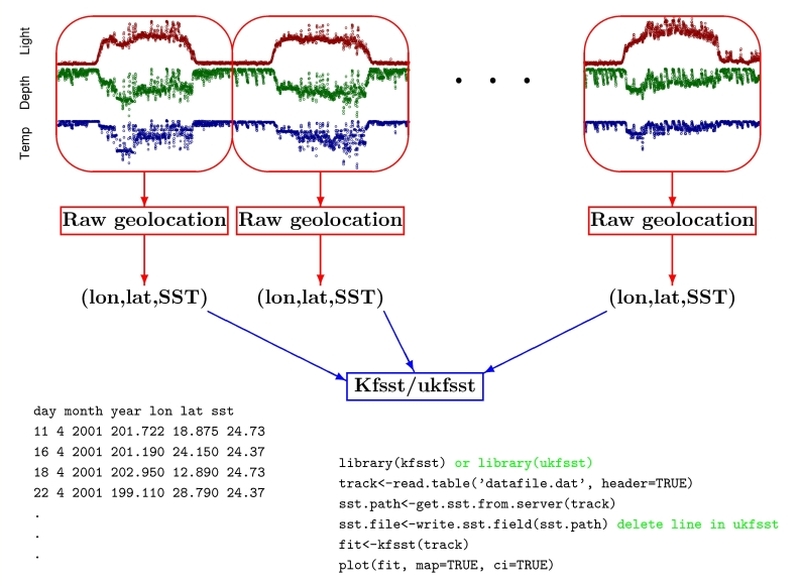

Cheatsheet of Ukfsst

Input data format

> track
   day month year  obsLon obsLat obsSst
    10     9 2002  198.04  23.09   30.6
    11     9 2002  198.11  50.50   30.7
    12     9 2002  197.65  45.50   30.6

Basic Workflow

# Note: delete the hash sign (#) at the beginning to uncomment a line

library(ukfsst)

# For users with R-3.1 and over, please run the following line as well:
# source('http://geolocation.googlecode.com/svn/trunk/support/ukfsst/func_ukfsst.r')
  
track<-read.table("datafile.dat", header=TRUE) # change file name and path for your own file
sst.path <- get.sst.from.server(track) 
# see function, get.blended.sst 
# for usage with higher-resolution SST imagery
fit<-kfsst(track)
plot(fit)

1. Read in a track
2. Obtain a corresponding SST-field
3. Reconstruct the track
4. Investigate the fitted track by plots and summaries

Handling tracks crossing from 360 to 0 longitude and vice versa

This problem will appear in the Eastern Atlantic when an animal crosses 0/360 longitude. Even though Ukfsst doesn't natively handle this problem, there is a getaround. It involves adding an offset to the raw longitude values to shift the longitude values to a continuous scale, instead of having a sharp break at 0/360. To achieve that, these are the steps:

1. Assume the raw data are in the -180 to 180 longitude system, e.g.,

  > head(track)
  day month year       lon      lat   sst
    9     1 2003 -75.01227 34.84846 21.30
   10     1 2003 -78.88831 38.14712 20.10
   11     1 2003 -78.28817 32.53389 19.10
   12     1 2003 -77.94039 26.73982 14.31
   13     1 2003 -77.84508 33.51983 16.50
   14     1 2003 -78.00233 39.64455 18.09
   
  > tail(track)
 day month year      lon      lat   sst
  28    10 2004 15.69613 32.13621 23.18
  29    10 2004 16.18055 27.32399 23.07
  30    10 2004 15.41815 29.59003 22.89
  31    10 2004 15.65907 29.82971 22.67
   1    11 2004 15.40330 30.06093 22.78
   1    11 2004 13.31000 40.74000 22.78

2. Add an offset to the input longitude values

  ### The modified longitude values need to stay within 0-360
  ### An offset of 200 is added here:
  
  myoffset = 200
  track$lon <- track$lon + myoffset
  maxlon = max(track$lon) + 10
  
  > range(track$lon)
  [1] 121.1117 216.1805
  > maxlon
  [1] 226.1805

3. Download SST images with an offset

• First use a modified SST download function

  source('http://geolocation.googlecode.com/svn/trunk/updates/get-reynolds.R')

• Input arguments include a request of SST data from 0 to 360 longitude, so that everything is downloaded
• Then apply an offset to the downloaded files, via the argument, offsetx
• Finally, trim extra SST data to keep files smaller and within bounds, via the argument, offset.cutoff

  sst.path<-get.reynolds(track[,c(3,2,1)], lonlow=0, lonhigh=360, latlow=18, lathigh=50,
                         minus180=T, offsetx= myoffset, offset.cutoff= maxlon)   

• Once download is complete, you are good to go!
• Lastly, make sure once you have obtained a fit, substract the offset from the fitted object.